Pipe to dot

Not all functions are pipe-friendly in every case: You may find some functions do not take your data produced by a pipeline as the first argument. In this case, you can enclose your expression by {} or () so that %>>% will use . to represent the value on the left and evaluate the enclosed expression.

For the linear model example, one can rewrite lm(formula = ) to

mtcars %>>%
  { lm(mpg ~ cyl + wt, data = .) }

# 
# Call:
# lm(formula = mpg ~ cyl + wt, data = .)
# 
# Coefficients:
# (Intercept)          cyl           wt  
#      39.686       -1.508       -3.191

or

mtcars %>>%
  ( lm(mpg ~ cyl + wt, data = .) )

# 
# Call:
# lm(formula = mpg ~ cyl + wt, data = .)
# 
# Coefficients:
# (Intercept)          cyl           wt  
#      39.686       -1.508       -3.191

The difference between {} and () used above is

1. {} accepts more than one expressions within the braces and its value is determined by the last one; but () accepts only one expression.
2. {} has only one feature: pipe to . in the enclosed expression while () has more features (we will cover them soon).

To demonstrate the difference, we run the following examples.

mtcars %>>% {
  model <- lm(mpg ~ wt + cyl, data = .)
  summ <- summary(model)
  summ[c("r.squared","adj.r.squared")]
}

# $r.squared
# [1] 0.8302274
# 
# $adj.r.squared
# [1] 0.8185189

It shows that {} holds a code block whose value is determined by the last expression or interrupted by return().

mtcars %>>% 
  lm(formula = mpg ~ wt + cyl) %>>%
  summary %>>% {
    if(.$r.squared >= 0.8) {
      return("Model A")
    }
    cat("Model B should be considered.\n")
    "Model B"
  }

# [1] "Model A"

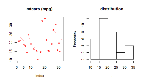
One thing to notice is that {} is more flexible than previously demonstrated. It also allows using %>>% within the braces as well as causing side effect such as plotting graphics.

mtcars %>>% {
  par(mfrow=c(1,2))
  .$mpg %>>% plot(col = "red", main="mtcars (mpg)")
  .$mpg %>>% hist(main = "distribution")
}

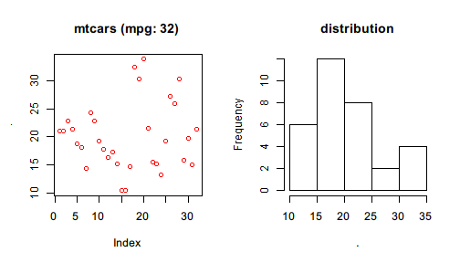
Another thing is that the meaning of nested dots are always determined by the working operator for that dot symbol. For example, the above code can be refined to

mtcars %>>% {
  par(mfrow=c(1,2))
  .$mpg %>>% plot(col = "red", main=sprintf("mtcars (mpg: %d)",length(.)))
  .$mpg %>>% hist(main = "distribution")
}

It should be obvious that . below par() belong to the first %>>% that works with mtcars while . in length() belong to the operator that works with .$mpg so that it can correctly show the length of mpg (32) rather than that of mtcars (11).

Creating closure

The expression will be evaluated with speically defined . if it is enclosed by {} or (). If an anonymous function, that is, a function definition without a name, is enclosed, the pipeline will result in a closure, a function returned by a function (%>>%) which can be used more times.

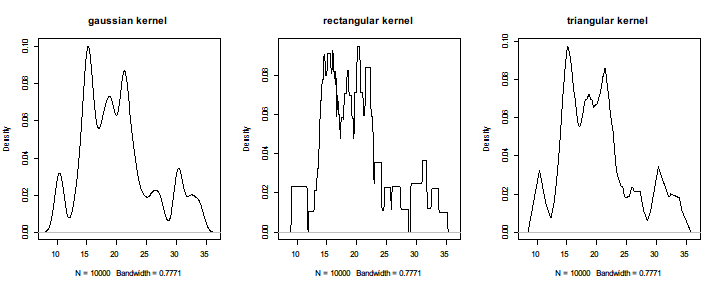
In the following example, we create a closure that takes one argument: the kernel method with which to perform the nonparametric density estimation of resampled mtcars$mpg.

density_plot <- mtcars$mpg %>>%
  sample(size = 10000, replace = TRUE) %>>%
  (function(kernel) {
    . %>>%
      density(kernel = kernel) %>>%
      plot(main = sprintf("%s kernel", kernel))
  })

We just create a closure called density_plot. Then we can call it with different kernels to see the differece between the density plots of each other.

par(mfrow=c(1,3))
density_plot("gaussian")
density_plot("rectangular")
density_plot("triangular")

However, if the enclosed function is called directly in the pipeline, %>>% will pipe the left value to its first argument because here the only difference between first-argument piping examples and this example is the function no longer has a name but created inline.

1:10 %>>% (function(x,pow) x^pow)(2)

#  [1]   1   4   9  16  25  36  49  64  81 100

A more complicated example is

mtcars %>>%
  lm(formula = mpg ~ wt + cyl) %>>%
  (function(model, warn_level) {
    if(summary(model)$r.squared < warn_level)
      warning("r.squared is too low", call. = FALSE)
    model
  })(0.9) %>>%
  coef

# Warning: r.squared is too low

# (Intercept)          wt         cyl 
#   39.686261   -3.190972   -1.507795

where an anonymous function is defined inline and %>>% following lm() pipes the linear model to the first argument of the anonymous function.